VLOOKUP - Quick Reference

Today i was using VLOOKUP after long (as was involved in Data Migration validation) and i kind of struggled a bit initially. It is straightforward once you know it, but if you have forgotten the mechanism and the logic behind it, it takes a few, not much, but a few iterations to get it right. The purpose of this quick reference blog post is to stop wasting the time in re-inventing the feature in future, if i not use it for long again. This is typical right, once you stop using what you have learnt, your brain tend to either delete it from your memory or keep it somewhere else in the memory, so that it can focus on the recent learning or tend to focus on what matters you most.

I am going to write this post in the language that i would understand once i refer to it in future.

VLOOKUP is simply finding a corresponding value for a desired constant, from a stack of huge data. For example, there may be a excel sheet with 10,000 rows and 19 columns. You know that 1st column is the list of employee id and all the other columns could have different set of data like, salary, leaves, role, employee name, project allocation, reporting manager and years of experience etc. 

Now if someone asks you to prepare a report for 2000 random employees out of 10,000 and they wish to include values from some random 8 columns out of 19, then there are potentially two ways to do it. Either manually search for each and every employee and then search for the corresponding values in the respective columns and then create the report, which is tedious and time consuming or simply use VLOOUP feature. 

Before using VLOOKUP, we shall first look at the contents of VLOOKUP.

VLOOKUP(lookup_value, table array, col_index_num, [range_lookup])

In our example, we will create a new excel sheet with first column being the employee ID (with employee IDs populated) and then the 18 columns for which we require the data. The next 18 columns is where we will be applying the VLOOKUP.

For example the first column is employee id and the first value in the employee ID column is 001 and is in cell A1.

Assume that we wish to find the employee name in the second column.We will apply the VLOOKUP in the second column i.e. Employee name .

The formula will be as follows:

VLOOKUP(A1, table array, col_index_num, [range_lookup])

lookup_value - will be the cell reference of the cell in which employee ID '001' resides, in the new result / report sheet.

table array - is the source of data where you are trying to find the corresponding value ( Employee name, in this case). In our case it will be the entire source sheet with 10,000 rows and 19 columns.

col_index_num - This is the most important parameter. This value is the COLUMN NUMBER from the SOURCE SHEET, where the desired values resides (desired value in this case is Employee name).

For example in the source sheet (with 10,000 rows and 19 columns), the first column is Employee ID and the employee name column is 12, counting from Employee ID, then the col_index_num value will be 12. This will tell the system to fetch the corresponding value from column 12 from the source sheet.

[range_lookup] - This value is either 0 (False, Exact match) or 1 (True, Approximate match). We will mostly (99% of the time) select 0, as hardly we will be interested in approximate value.

But to explain this in more detail, please look at the example below:

In the screenshot below, we are trying to find the value for '2'. However '2' is not present in source data. In this case, if the  [range_lookup] value is '0' .i.e. Exact match (False), then the system displays an '#N/A' error.

[range_lookup] value is '0', col_index_num value = '3' (as 'L' is 3 columns away from 'J')

No 'EXACT' value for '2' hence error is displayed '#N/A'

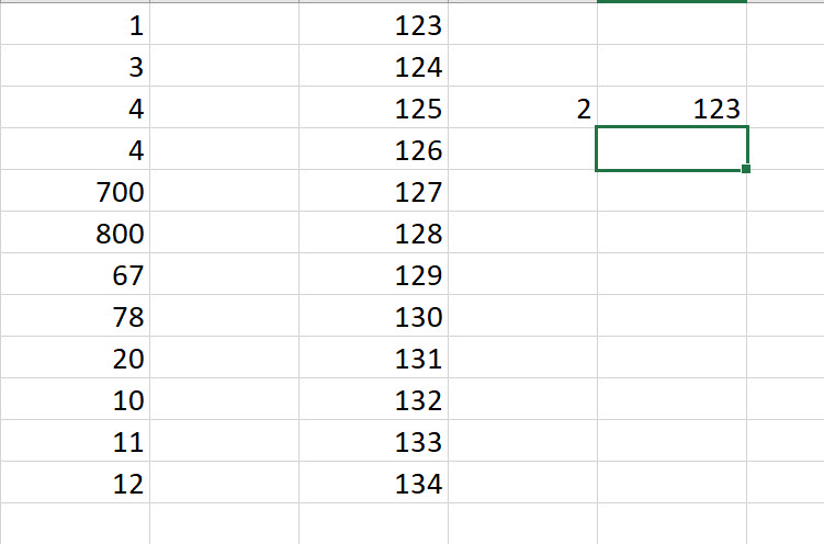
Now if the [range_lookup] value is changed to '1', the system will return the next largest value, that is less than your specific lookup value. In this case it is '123'.

[range_lookup] value is '1', col_index_num value = '3' (as 'L' is 3 columns away from 'J')

No 'APPROXIMATE' value for '2' is found, hence largest value less than to the corresponding look up value (which is value against '1' in this case) is displayed, which is '123'

This is quick reference for VLOOKUP, for me. Hope i will not have to use this post again to remind me of VLOOKUP. But if at all i had to, this post should help me refresh the learning and i should hopefully spend less time reinventing this functionality in future.

Thanks

Sarang